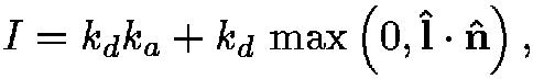
where I is the RGB color to be displayed for a given point on the
surface, kd is the RGB diffuse reflectance at the point, ka is
the RGB ambient illumination, is the unit vector in the
direction of the light source, and is the unit surface normal
vector at the point. This model is shown for kd = 1 and ka = 0
in Figure 4.13.
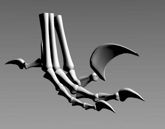
This unsatisfactory image hides shape
and material information in the dark regions. Both highlights and
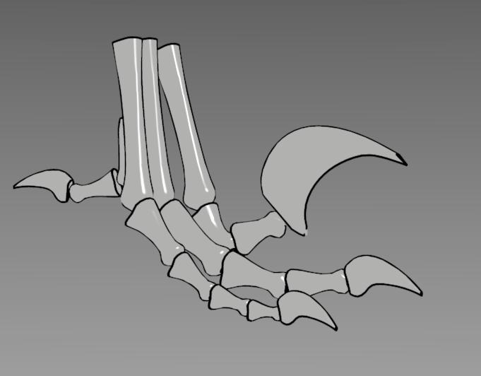
edge lines can provide additional information about the object. These
are shown alone in Figure 4.14 with no shading. Edge
lines and highlights could not be effectively added to
Figure 4.13 because the highlights would be lost in the
light regions and the edge lines would be lost in the dark regions.
|
| Figure 4.13: Diffuse shaded image using Equation 4.1 with kd = 1 and ka = 0. Black shaded regions hide details, especially in the small claws; edge lines could not be seen if added. Highlights and fine details are lost in the white shaded regions. |
|
| Figure 4.14: Image with only highlights and edges. The edge lines provide divisions between object pieces and the highlights convey the direction of the light. Some shape information is lost, especially in the regions of high curvature of the object pieces. However, these highlights and edges could not be added to Figure 4.13 because the highlights would be invisible in the light regions and the silhouettes would be invisible in the dark regions. |
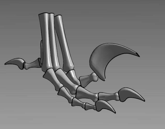
To add edge lines to the shading in Equation 4.1, either of two standard heuristics could be used. First ka could be raised until it is large enough that the dim shading is visually distinct from the black edge lines, but this would result in loss of fine details. Alternatively, a second light source could be added, which would add conflicting highlights and shading. To make the highlights visible on top of the shading, kd could be lowered until it is visually distinct from white. An image with hand-tuned ka and kd is shown in Figure 4.15. This is the best achromatic image using one light source and traditional shading. This image is poor at communicating shape information, such as details in the claw nearest the bottom of the image, where it is colored the constant shade kd ka regardless of surface orientation.
|
| Figure 4.15: Phong-shaded image with edge lines and kd = 0.5 and ka = 0.1. Like Figure 4.13, details are lost in the dark gray regions, especially in the small claws, where they are colored the constant shade of kd ka regardless of surface orientation. However, edge lines and highlights provide shape information that was gained in Figure 4.14, but could not be added to Figure 4.13. |