Tone-based Shading of Matte Objects

 

In a colored medium such as air-brush and pen, artists often use both hue and luminance (grayscale intensity) shifts. Adding black and white to a given color results in what artists call shades in the case of black and tints in the case of white. When color scales are created by adding gray to a certain color they are called tones  [3]. Such tones vary in hue but do not typically vary much in luminance. Adding the complement of a color can also create tones. Tones are considered a crucial concept to illustrators and are especially useful when the illustrator is restricted to a small luminance range [21]. Another quality of color used by artists is the temperature of the color. The temperature of a color is defined as being warm (red, orange, and yellow), cool (blue, violet, and green), or temperate (red-violets and yellow-greens). The depth cue comes from the perception that cool colors recede whereas warm colors advance. In addition, object colors change temperature in sunlit scenes because cool skylight and warm sunlight vary in relative contribution across the surface, so there may be ecological reasons to expect humans to be sensitive to color temperature variation. Not only is the temperature of a hue dependent upon the hue itself, but this advancing and receding relationship is effected by proximity [5]. Gooch et al. used these techniques and their psychophysical relationship as the basis for their shading model.

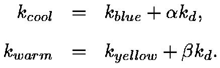
The classic computer graphics shading model can be generalized to experiment with tones by using the cosine term (l . n) of Equation 4.1 to blend between two RGB colors, k_cool and k_warm:

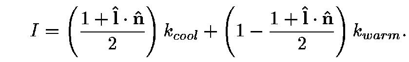
Note that the quantity l . n varies over the interval [-1,1]. To ensure the image shows this full variation, the light vector l should be perpendicular to the gaze direction. Because the human vision system assumes illumination comes from above [14], it is best to position the light up and to the right and to keep this position constant.

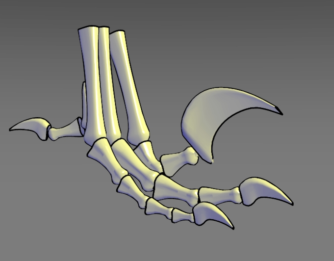
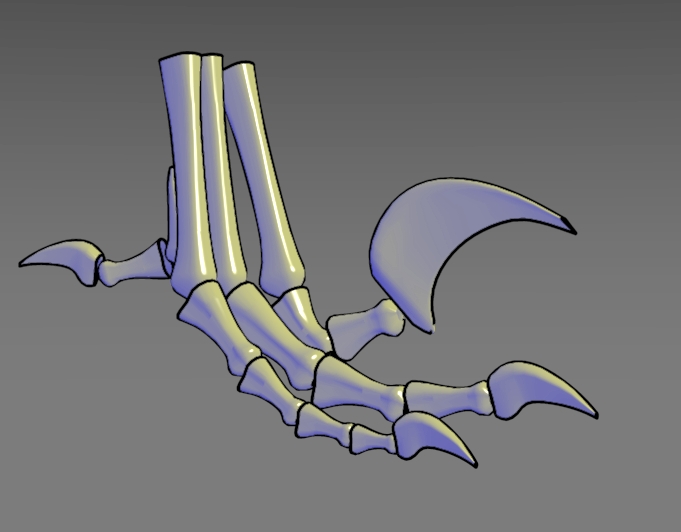
An image that uses a color scale with little luminance variation is shown in Figure 4.16.

  

Figure 4.16: Approximately constant luminance tone rendering. Edge lines and highlights are clearly noticeable. Unlike Figures 4.13 and 4.15 some details in shaded regions, like the small claws, are visible. The lack of luminance shift makes these changes subtle.

This image shows that a sense of depth can be communicated at least partially by a hue shift. However, the lack of a strong cool-to-warm hue shift and the lack of a luminance shift makes the shape information subtle. The unnatural colors may also be problematic. The colors chosen for this hue shift must be picked with care. A red-green hue shift would be undesirable because of red-green color blindness. A blue-yellow hue shift is most common in many art forms and may be most natural because of yellow sun-light and shadows lit by the ambient blue sky. Blue and yellow, having a very large intensity shift, will also provide the desired luminance shift.

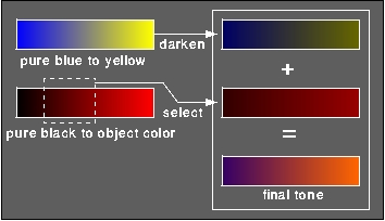
In order to automate this hue shift technique and to add some luminance variation to the use of tones, Gooch et al. examined two extreme possibilities for color scale generation: blue to yellow tones and scaled object-color shades. The final model is a linear combination of these techniques. Blue and yellow tones are chosen to insure a cool to warm color transition regardless of the diffuse color of the object.

The blue-to-yellow tones range from a fully saturated blue: k_blue = (0,0,b), b is in the range [0,1] in RGB space to a fully saturated yellow: k_yellow = (y,y,0), y is in the range [0,1] . This produces a very sculpted but unnatural image and is independent of the object's diffuse reflectance k_d. The extreme tone related to k_d is a variation of diffuse shading where k_cool is pure black and k_warm = k_d. This would look much like traditional diffuse shading, but the entire object would vary in luminance, including where l . n < 0. A compromise between these strategies will result in a combination of tone scaled object-color and a cool-to-warm undertone, an effect which artists achieve by combining pigments. The undertones can be simulated by a linear blend between the blue/yellow and black/object-color tones:

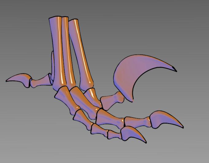
Plugging these values into Equation 4.1 leaves four free parameters: b, y, alpha, and beta. The values for b and y will determine the strength of the overall temperature shift, and the values of alpha and beta will determine the prominence of the object color and the strength of the luminance shift. In order to stay away from shading which will visually interfere with black and white, intermediate values should be supplied for these constants. An example of a resulting tone for a pure red object is shown in Figure 4.17.

  

Figure 4.17:How the tone is created for a pure red object by summing a blue-to-yellow and a dark-red-to-red tone.

Substituting the values for k_cool and k_warm from Equation 4.1 into the tone Equation 4.1 results in shading with values within the middle luminance range as desired. Figure 4.18

  

Figure 4.18: Luminance/hue tone rendering. This image combines the luminance shift of Figure 4.13 and the hue shift of Figure 4.16. Edge lines, highlights, fine details in the dark shaded regions such as the small claws, as well as details in the high luminance regions are all visible. In addition, shape details are apparent unlike Figure 4.14 where the object appears flat. In this figure, the variables of Equation 4.1 and Equation 4.1 are: b = 0.4, y = 0.4, alpha = 0.2 and beta = 0.6. .

is shown with b = 0.4, y = 0.4, , alpha = 0.2 and beta = 0.6 . To show that the exact values are not crucial to appropriate appearance, the same model is shown in Figure 4.19 with b= 0.55, y = 0.3, alpha = 0.25, and beta = 0.5. Unlike Figure 4.15, subtleties of shape in the claws are visible in Figures 4.18 and  4.19.

  

Figure 4.19: Luminance/hue tone rendering, similar to Figure 4.18 except b = 0.55, y = 0.3, alpha = 0.25, and beta = 0.5. The different values of b and y determine the strength of the overall temperature shift, where as and determine the prominence of the object color, and the strength of the luminance shift.

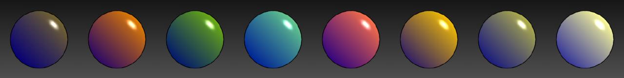
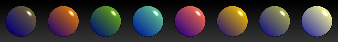
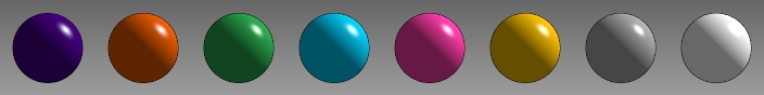
The model is appropriate for a range of object colors. Both traditional shading and the new tone-based shading are applied to a set of spheres in Figure 4.20. Note that with the new shading method objects retain their ``color name'' so colors can still be used to differentiate objects like countries on a political map, but the intensities used do not interfere with the clear perception of black edge lines and white highlights. One issue that is mentioned as people study these sphere comparisons is that the spheres look more like buttons or appear flattened. I hypothesize a few reasons why this may be so. The linear ramp of the shading may be too uniform and cause the spheres to flatten. The shading presented here is just a first pass approximation to the shading artists use and much improvement could be made. Another problem may be that the dark silhouettes around to the object may tie the spheres to the background. Figure 4.21 shows three sets of spheres, shaded the same but put against different gradations of background. The edge lines of the spheres on the darkest background fade a little bit and even seem to thin towards the light, due to the gradation of the background. In my opinion, the spheres set against the darkest background, where the edge lines loose some emphasis, seem to be a little more three dimension than the spheres with edge lines.

  

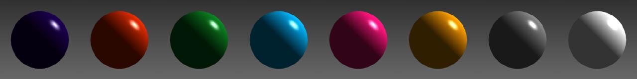
Figure 4.20: Comparing shaded, colored spheres. Top: Colored Phong-shaded spheres with edge lines and highlights. Bottom: Colored spheres shaded with hue and luminance shift, including edge lines and highlights. Note: In the first Phong-shaded sphere (violet), the edge lines disappear, but are visible in the corresponding hue and luminance shaded violet sphere. In the last Phong-shaded sphere (white), the highlight vanishes, but is noticed in the corresponding hue and luminance shaded white sphere below it. The spheres in the second row also retain their ``color name.''

  

Figure 4.21: Tone and undertone shaded spheres with backgrounds getting darker.

  

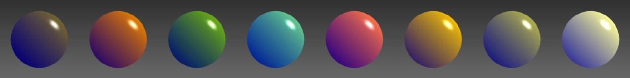
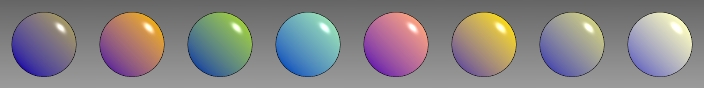
Figure 4.22: Shaded spheres without edgelines. Top: Colored Phong-shaded spheres without edge lines. Bottom: Colored spheres shaded with hue and luminance shift, without edge lines.

Figure 4.22 shows both the Phong-shaded spheres and the spheres with new shading without edge lines. Without the edge lines, the spheres stand out more. Spheres are not really the best model to test this new shading and edge lines. Edge lines are not really necessary on a sphere, since edge lines are used by illustrators to differentiate parts and discontinuities in a model, something that is not really necessary in a simple model like a sphere. However, it is a computer graphics tradition to test a shading model on the spheres.