|
Fluid Modeling
|
Rather than writing my own simulator from scratch,
I began work on this project by hunting around on the web to get a sense of
what had already been done in the area of 2d fluid simulation, and how much
code was already freely available. I discovered that there are a quite a few
simple 2d fluid simulators floating around out there. As far as I have seen,
every one of them is based on the semi-Lagrangian simulation method introduced
by Jos Stam in Stable Fluids. I found source code for three such fluid
demos; all of which performed the diffusion and projection steps using Fourier
transforms in the way suggested by Stam. Unfortunately, I aspire to create
a fluid simulator which can be used in my non-photorealistic rendering project,
and thus I really want to be able to render fluids bounded to arbitrary volumes.
And this is too bad, as the Fourier transform technique only works given periodic
boundaries.
Stam outlines a second approach to dealing with the diffusion and project
steps, in which a sparse linear solver is used instead of the FFT. Unlike
the FFT method, the linear solver based simulation can in principle be modified
to work with any boundary conditions. And luckily for me, Stam recently made
a stripped down version of the linear programming-based solver available on
his website. I have used this solver, rather than any of the FFT based demos,
as the starting point for my own work.
Stam's solver assumes that the fluid is bounded by a rectangle. I have altered
his code to implement a more general bounding method in which a boolean grid
is used to specify certain areas as off limits to fluid flow. The velocity
field inside of the blocked off areas is set to zero; combined with the modified
particle tracing method discussed below, this will stop any matter from moving
through the blocked off areas. At the same time, the density fields inside
of the blocked off areas are assumed to be the same as the density fields
immediately outside of the areas; this prevents material from diffusing into
or out of the blocked zones. In the current version of my code, the density
of a blocked off square is set to the average of all surrounding non-blocked
off squares. Unfortunately, this method only works if all boundaries are at
least 2 squares thick. A better way to do things is to change all parts of
the code in which the density in a square's neighbor is checked such that
the square's own value is used in the case that the neighboring square is
blocked. Thus, if the square below a blocked square checks the blocked square's
value, it sees something different than when the square above checks it. That
method, while slightly more difficult to implement, has the advantage of allowing
single width squares to be blocked off, and slightly improves fluid behavior
at corner points (where there have to be at least 2 unblocked squares neighboring
a single blocked square).
My first attempt at bounding areas used the ambitious "thin boundary" approach
described above, but it was plagued by strange behaviors. I scaled back to
the more modest averaging approach (which seems to work perfectly well in
practice and allowed me to get away with using a very simple particle tracer).
At first the averaging approach also showed problems. Eventually I traced
those problems back to an asymmetry in Stam's implementation of the Gauss-Seidel
relaxation solver. After a slight modification to the solver the bounding
method seems to work fine. The modification involved creating a relaxed version
of the entire matrix, and then replacing all the old values at the same time
(Stam's code just puts the relaxed values directly into the target matrix).
Now that the linear solver issue has been sorted out, I am tempted to take
another shot at the thin boundary method.
Besides forcing some areas of the velocity and density grids to certain values,
implementing the boundary constraints also requires a modification in the
advection step. In Stable Fluids, advection is calculated by tracing
a particle positioned at each square's center back along the velocity field
to see where it would have been at the end of the last time step. The easiest
way to do this is to linearly interpolate the particle's position using its
current velocity. In other words,
p_old=p_current * (-v).
However, once arbitrary boundaries get thrown into the mix, this approach
will no longer work, as you need to make sure that high velocity particles
don't move through a boundry area.
The "right" way to do this would be to use some line intersection
point equations to find the exact point at which any particle's trajector
intersected the edge of one of a boundry region, and then declaring the old
particle position to be that intersection point (this is basically the method
outlined used in Visual Simulation of Smoke). A more ambitious variation
on this approach would assume that the particle bounced off the boundary edge,
rather that just stopping at the intersection point (you would probably want
to assume an elastic collision with the boundry). Of course, if you are trying
to make a high precision simulation, using linear interpolation to find old
particle positions is troublingly inaccurate. Before going to the trouble
to calculate particle bounces, you would want to switch to more precise curve-based
interpolator, such as the monotonic cubic interpolator used in Visual Simulation
of Smoke.
However, the particle tracing method that I settled on never performs an explicit
intersection test. I just calculate how much time will be required for the
particle to move half a square-width given its current speed, and do a linear
interpolation using that value as my delta-t. I then recalculate the particle's
velocity based on its new position in the velocity field, and repeat this
pattern until I don't have enough time left to make it another half square
width. Then I use up the remainder of my time on one last linear interpolation.
The method ensures that I never travel through boundaries (since they are
all 2 squares worth of zero velocity points and I am only moving half a square
width at a time). Because the density values inside of each boundary are set
to the averages of their neighbors, the values that my advection step ends
up returning are very nearly those that would have been returned, had the
tracer stopped at exactly the boundary edge.
In addition to arbitrary boundaries, I've implemented vorticity confinement,
as described in Visual Simulation of Smoke. While they are wonderfully
stable, semi-Lagrangian fluid simulations are known to suffer from numerical
damping. More specifically, the velocity field in the simulation losses it
curl too quickly. Therefore any vortices which form die away more quickly
than they should. The technique of vorticity confinement simply adds in a
force which acts to replace the lost curl. This technique is especially nice
to have implemented when one is using a fluid simulator in the context of
non-photorealistic rendering. By magnifying the confinement forces far beyond
what is physically reasonable, you can create velocity fields in which the
effects of turbulence are greatly exaggerated; just the sort of thing you
want if you are trying to imitate Van Gogh's painting style.
My simulation runs inside of a wx OpenGl application, much like that developed
for my first assignment. It provides menus and dialogs which allow me to edit
just about every constant of the simulation. The same program also servers
as an interface for all of my NPR algorithms.
Because a Stam style semi-Lagrangian simulator keeps matter density values
neatly separate from the calculation of the velocity fields, it is easy to
modify the algorithm to allow for many different density matrices. You can
think of this as having a simulation in which there are several different
dyes which can be injected into pool of water. Each dye represents one of
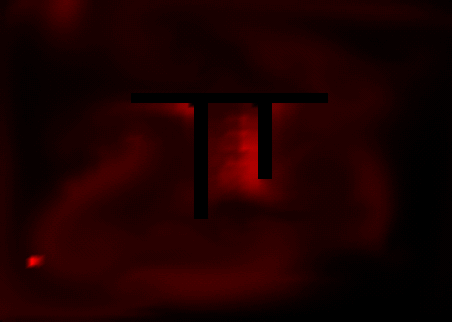
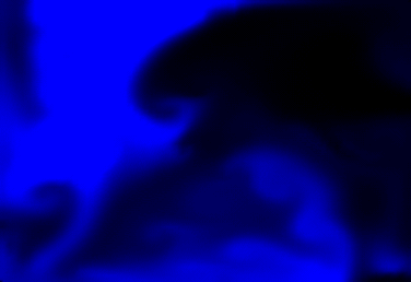
the density matrices. As I currently have things setup, I keep track of four
different dyes, each of which is rendered with its own color (red, green,
blue, and white).
 Here's a screenshot taken of a 2 dye simulation. I had fun
making this image; I turned the viscosity way up so that after I had finished
messing around with one patch of dye, it would stay more or less in place.
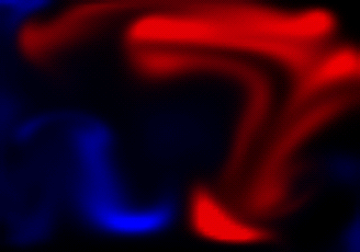
Here's a screenshot taken of a 2 dye simulation. I had fun
making this image; I turned the viscosity way up so that after I had finished
messing around with one patch of dye, it would stay more or less in place.
Because it allows me to create some pretty effects, I have also added constants
for dye brightness, which exaggerates the color of the dyes by a multiplicative
constant, and dye decay. Each value in the density matrix is multiplied by
the decay value after every time step, I usually set this to something like
.99 just too keep the simulation from becoming excessively "muddied" by completely
diffused dyes.
The things I yet to get around to:
While it does do a good job of letting me control all the constants of the
simulation, I would like to extend the UI that I have built such that I can
specify more interesting fluid elements. For example, I would like be able
to specify areas of the grid which are matter sources or sinks, and well as
areas in which the velocity field is set to an arbitrary value. These features
could be immediately applied to creating nice looking NPR renderings.
Most of the key pieces of the simulation are one dimensional algorithms, and
the rest (such as the particle tracer) can be easily moved from 2d to 3d.
For that reason, I had been planning to make a 3d version of the simulator,
but as it wasn't terribly useful to my NPR work, the 3d simulator has always
been a low priority, and I have yet to get around to it. In Visual Simulation
of Smoke, Fedkiw uses linear solvers more sophisticated than the relaxation
based algorithm included in Stam's code. Following a comment in one of Stam's
papers, I've gotten my hands on the NIST implementations of some better linear
solvers, though I hadn't planned to plug them in until after making the jump
to a 3 dimensional simulation.
I really don't have much interested in simulating smoke per say- I prefer
to think of the simulation as dyes transported in water. However, with a little
bit of renaming, I could get myself very close to Fedkiw's smoke simulation.
If I designate one of my dyes to be "smoke particles", and another one to
be "temperature", then adding the temperature and gravity based forces given
in Visual Simulation of Smoke into my simulation should be easy.
While simulating smoke should be pretty simple, what I would really like to
do is to find a way to add some forces, based on dye concentration, that would
act to discourage mixing between dyes. If governed by the right equation set,
these kinds of "oil in water" effects would be ideal material for my NPR renderings.
Links:
My Much Mentioned NPR Project
Project source code
- Distributed as a stripped snapshot of my dev
directory; just about all of the code involved in the simulator lives in dev/fluids.
Jos Stam,
Stable Fluids.
- The original semi-Lagrangian paper.
Ronald Fedkiw, Jos Stam, and Henrik Jensen, Visual
Simulation of Smoke.
- Vorticity confinement
Jos Stam, Real-Time Fluid Dynamics for
Games.
- This paper was apparently presented at a recent
game programming conference, the code
provided with it forms the base of my own simulator.
Patrick Witting, Computation Fluid
Dynamics in a Traditional Animation Environment.
- A recent Fluid simulation paper that is NOT
based on semi-Lagrangian methods, the simulation presented takes into account
many forces that Stam's does not, in particular, some pressure effects that
I would love to somehow incorporate into my own solver.
Gustav Taxen's Solver
- This is the classic FFTW-based semi-Lagrangian
implementation.
Nvidia's fluid
Demo
- Based on Gustav's code, though it include
a somewhat prettier rendering method.
John DeWeese and Kumar Iyer's
FFTW based solver
- I found that I needed to use the version of
the FFTW libs distributed with this program in order to make working builds
of Nvidia's and Gustav's code.
Andrew Selle
- Another student who seems to have walked many
of the same paths as I have.
Line intersection tests
-This describes the line intersection-point
equations that I considered using in my particle tracing algorithm. There
are situations (say if you want to simulate bounding areas represented by
arbitrary polygons), in which particle tracing that made use of these sorts
of intersection algorithms would lead to faster and more accurate simulations
than my current tracing method.
|
|
|