Srf-Node Method

The Srf-Node Method is the most concise. Nodes correspond to parameter values which are the average of consecutive sets of (order-1) knots from the knot vector, ignoring the first and last ones. There are exactly the same number of nodes as there are control points. It is often convenient to use the nodes when a parameter value or point on the curve needs to be associated with a control point [19].

A normal is calculated for every node point on a surface, as shown in Figure 4.4(b). This calculation can be done as a preprocess and only has to be done once per surface.

Then, E(u,v) . n(u,v) is calculated for every view and every node point, where n(u,v) is the surface normal at the node point and E(u,v) is the vector from the eye to the point on the surface. The resulting signs of the dot products, , are stored in a table, one per node point, as shown in Figure 4.8. If is zero then there is a silhouette at that node point on the surface. By searching the table in the u direction and then in the v direction, a silhouette can be found by comparing to _{i+1, j} and to _{i, j+1} , respectively. If a sign changes from + to - or from - to +, then there is a silhouette between those two points on the surface, as shown in Figure 4.4(b).

  

Figure 4.8: Visualize the Srf-Node Method as a table of signs

, where can be +, -, or 0.

When a region containing a silhouette point is found between two node points, it is linearly interpolated, as shown in Figure 4.1. The interpolation is based on two surface points and the respective angles formed by the normal and the eye vector, calculated as in Equation 4.1 and 4.1 and as discussed in Section 4.1.2.1.

  

Figure 4.9: Srf-Node Method can result in missed silhouettes depending upon the node points. If for example, the node points were those that correspond to theta_1, theta_2,and theta_3, there would be three missed silhouette points because theta_1, theta_2,and theta_3, are all less than 90 degrees and there would be no sign change. However, if the nodes points were alpha, theta_2,and theta_3, then alpha is greater than 90 degrees and theta_2 is less than 90 degrees, so the silhouette between the two corresponding node points would not be missed and could be interpolated. The problem of missing these silhouettes can be remedied by refining the control mesh.

In order for this method to work, the surface has to be sufficiently refined or it may miss silhouettes, as discussed in Figure 4.9. Surface refinement only needs to be done once and can be done as a preprocess over the whole surface. However, the refinement increases the number of control points and thus the number of checks necessary to locate the silhouette points. It may be better to refine the area where a silhouette may be, based on testing the control mesh.

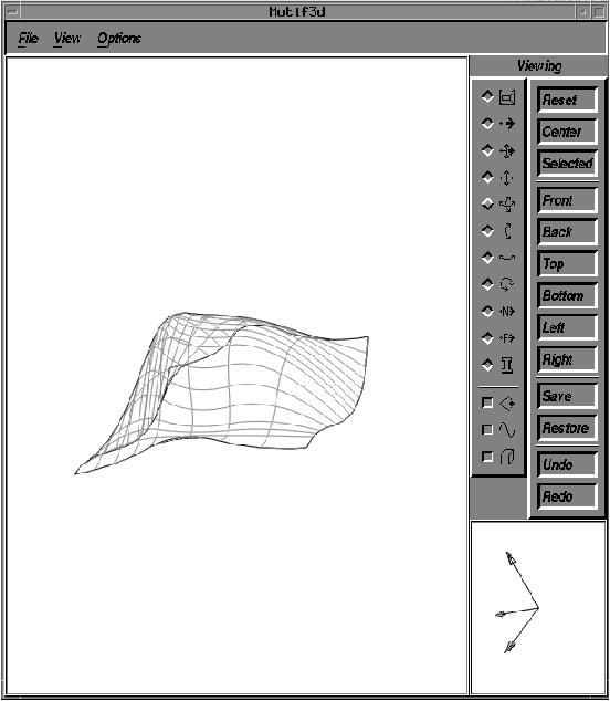
Using a 2D marching-cube data structure makes it easy to connect the silhouette points to form linear silhouette curves. Figure 4.5(b) provides a visualization of the and the approximate silhouette lines. This method results in edge lines as displayed in Figure 4.10. Another exaple is shown in the top down view shown in Figure 4.11 and the view from the eye point in Figure 4.12.

    

View of surface with silhouettes and surface boundaries generated with Srf-Node Method.	Looking down on surface with silhouettes and surface boundaries.
Figure 4.10: Srf-Node Method.

  

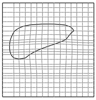
Figure 4.11: Looking down on surface with silhouette generated with Srf-Node method. Compare this image with the 2D projection and approximation of silhouettes shown in Figure 4.5 using the Mesh method and the Srf-Node method.

  

Figure 4.12: View of the same surface represented in Figure 4.5,  4.4, and 4.11 with silhouettes generated with the Srf-Node method.